Model comparison for ziplss GAMs by automatically generating all nested models and running them in parallel.
Introduction
Statistical models are used commonly in ecology to improve our understanding of ecological dynamics and processes. At their foundation, these models quantify the relationships between a response variable and a suite of explanatory covariates. These covariates can be observational or environmental and are described in linear or non-linear fashion, depending on the modeling approach. However, determining which covariates to include in a model can be a bit tricky. One of the most commonly-accepted methods to determine a model formula is through AIC model comparison and averaging of nested models within a global model. A global model is one that is fully-defined with the inclusion of all considered covariates, while nested models include only a subset of those covariates. Although a global model includes more information, nested models sometimes perform better, as predicted by the principle of parsimony. Also known as Occam’s Razor, this principle states that the simplest explanation is often correct, supporting the case for a more parsimonious model (Stoica & Söderström 1982, and for a recent discussion on this topic, see: Coelho et al. 2019). This necessitates the model comparison process; otherwsie we would always build and select a model with the greatest number of covariates.
Generating a set of nested models from a global model is typically automated in popular statistical softwares (such as Program MARK for ecologists), but this primarily applies to linear models. However, as many biological relationships are nonlinear, models that can more accurately describe such relations have become increasingly prominent in scientific literature. One of the most popular methods to model nonlinear relationships is with Generalized Additive Models (‘GAMs’). GAMs are a powerful tool in all analytical fields and have been used to predict things from the trajectory of stock markets to changes in species distributions under climate change emissions scenarios.
Personally, my experience with GAMs is from my undergraduate thesis on avian populations and West Nile virus, where I used a GAM to construct a spatiotemporal model of count data from Project FeederWatch. It was a special type of model known as a Zero Inflated Poisson Location-Scale Model (‘ziplss’ or ‘ZIP(LSS)’), as developed by the highly-regarded Dr. Simon Wood (Wood et al. 2016). This ziplss GAM is a hierarchical model separated into two stages: the first stage models the probability of presence, while the second stage models the average abundance given presence. From a biological perspective, it allows us to ask: 1) is an individual detected? and 2) if so, how many of them are there? (Robinson et al. 2018, Appendix 2)
This is all well and good, but the two-stage strcutre of the model formula makes it far more difficult to generate and test all nested models. However, this is a necessary part of the process, especially as step-wise model selection (which works in the other direction) has become less accepted. I’ve written this tutorial on how to go about this process for the ziplss GAM, hoping it’s useful to others in the field and can be applied to other models, as well. Additionally, I’ll include the model comparison process, which makes use of parallel computing to speed up the process. This is increasingly useful as more explanatory variables are included, as fitting GAMs is computationally intensive, and therefore, time-consuming. In this case, parallelizing the process allows for each core in a cluster to run a model, so that multiple models can run simultaneously across all assigned cores. On my computer, I have 16 cores, 15 of which I add to a cluster, allowing me to run 15 GAMs simultaneously, which greatly reduces the run-time of the program.
Methods
Borrowing simulated data for reproducibility
It’s important to have reproducible data in a tutorial like this, as it allows others to have an easier time following the code. The model we’ll be working with is fairly niche and the typical reproducible example data sets (mtcars, iris) don’t quite fit. However, the developer of the ziplss model provided some code that allows us to simulate data for modeling. This first chunk is borrowed directly from the mgcv vignette (Wood et al. 2016).
set.seed(1)
## simulate some data...
f0 <- function(x) 2 * sin(pi * x); f1 <- function(x) exp(2 * x)
f2 <- function(x) 0.2 * x^11 * (10 * (1 - x))^6 + 10 *
  (10 * x)^3 * (1 - x)^10
n <- 500;set.seed(5)
x0 <- runif(n); x1 <- runif(n)
x2 <- runif(n); x3 <- runif(n)

## Simulate probability of potential presence...
eta1 <- f0(x0) + f1(x1) - 3
p <- binomial()$linkinv(eta1)
y <- as.numeric(runif(n)<p) ## 1 for presence, 0 for absence

## Simulate y given potentially present (not exactly model fitted!)...
ind <- y>0
eta2 <- f2(x2[ind])/3
y[ind] <- rpois(exp(eta2),exp(eta2))
The rest of this tutorial is my own original code.
Setup
First, we’ll load the required packages. The mgcv package is the leading package for fitting GAMs in R, tidyr greatly improves coding efficient by tapping into the tidyverse framework, stringr allows for better methods to manipulate strings, and qpcR provides some neat functionality for model comparison.
library(mgcv)
library(tidyr)
library(stringr)
library(qpcR)
We’ll store the simulated data into a data.frame, which helps to keep things straight. Notice that beyond the five simulated variables, we also included an invariant term, which is simply a column downfilled by 1s that we’ll make use of later. Be sure to add this column to your data.
df = data.frame(
  y  = y, # response
  x0 = x0, # detect
  x1 = x1, # detect
  x2 = x2, # count
  x3 = x3 # count
)

df$invar = 1 # invariant term
We can print the first five rows of this data.frame using the head() function, allowing us to get a sense for the data.
head(df, 5)
      y        x0        x1        x2        x3 invar
    1 4 0.2002145 0.3981236 0.4662433 0.5097162     1
    2 0 0.6852186 0.1971769 0.3769562 0.9663678     1
    3 0 0.9168758 0.3947733 0.5788920 0.1742736     1
    4 5 0.2843995 0.6230317 0.6161464 0.1609478     1
    5 1 0.1046501 0.5651958 0.8906188 0.5039395     1
Generating all possible covariate combinations
In a single function, we’ll specify all of the explanatory variables for both stages of our global model and then generate all the possible combinations of those variables. We can do this using the expand.grid() function, which generates the Cartesian product of the supplied values. Although our end goal is to create a model formula, exapand.grid() outputs a data.frame object, where each row represents a nested model equation. We’ll convert these rows to formulas in the next step.
count = expand.grid(
  count_x2  = c("s(x2)", "invar"),
  count_x3  = c("s(x3)", "invar")
)

detect = expand.grid(
  detect_x0  = c("s(x0)", "invar"),
  detect_x1  = c("s(x1)", "invar")
)
This gives us the following output:
print(count)
      count_x2 count_x3
    1    s(x2)    s(x3)
    2    invar    s(x3)
    3    s(x2)    invar
    4    invar    invar
print(detect)
      detect_x0 detect_x1
    1     s(x0)     s(x1)
    2     invar     s(x1)
    3     s(x0)     invar
    4     invar     invar
In both stages, all covariates are fully-defined in the first row and the following rows represent scenarios where a covariate is effectively removed. Looking at the count stage, we see that in the second row, x2 becomes invariant, but in the third row, x3 becomes invariant, and in the fourth row, both terms become invariant.
Converting to model formulas
The next part of this code is a bit less straightforward. In the first line we create alist vector with 256 blank elements, which is the total number of models we’ll test (1 global + 255 nested). This is because there are four parameters with two options (variant vs invariant) in each of the two steps, so: $2^2 * 2^2 = 16$. The model formulas need to be saved in a list form as this is what the mgcv::gam() function expects.
We set k = 1 as the initial position for iteration through the nested loops. We then loop through both stages of the model, unlisting each row from the data.frame and converting it to a character vector. During this process, the selected parameters are concatenated with a + symbol to follow the syntax expected by the mgcv::gam() function. The final model uses ~ in concatenating both stages from the i and j loops, and again uses ~ to specify the response (here, maxFlock).
Finally, k = k + 1 increments the process through the 16 iterations.
model.formulas = vector("list", 16)
k = 1
for (i in 1:length(count[, 1])) {
  a = as.character(unlist(count[i, ])) %>%
    str_flatten(collapse = " + ")

  for (j in 1:length(detect[, 1])) {
    b = as.character(unlist(detect[j, ])) %>%
      str_flatten(collapse = " + ")

    model.formulas[[k]] = list(formula(str_glue("y", " ~ ", a)),
                               formula(str_glue(" ~ ", b)))
    k = k + 1
  }
}
Printing the first item in the list results in the appropriately-formatted model formula of the global model.
print(model.formulas[[1]])
    [[1]]
    y ~ s(x2) + s(x3)

    [[2]]
    ~s(x0) + s(x1)
In the resulting formula for the global model shown above, we see that the structure is a nested list, where model.formulas[[1]][[1]] is the count stage and model.formulas[[1]][[2]] is the detection stage. These formulas are now ready to be used in the mgcv::gam() function.
Generating model names
The next step uses the same code structure as the previous segment, but instead of concatenating model formulas, we’ll generate the model names.
count.names = expand.grid(
  count_x2  = c("x2", "."),
  count_x3  = c("x3", ".")
)

detect.names = expand.grid(
  detect_x0  = c("x0", "."),
  detect_x1  = c("x1", ".")
)

model.names = vector("list", 16)
k = 1
for (i in 1:length(count.names[, 1])) {
  a = as.character(unlist(count.names[i, ]))
  a = paste(a, collapse = ",")

  for (j in 1:length(detect.names[, 1])) {
    b = as.character(unlist(detect.names[j, ]))
    b = paste(b, collapse = ",")

    model.names[[k]] = paste(str_glue("N(", a, ")", "Phi(", b, ")"))
    k = k + 1
  }
}
And again, we can see the results below, where the first model name represents the full model, and the next two model names represent models with the substitution of invariant terms in the detection portion, representing the first of the nested models.
head(model.names, 3)
    [[1]]
    [1] "N(x2,x3)Phi(x0,x1)"

    [[2]]
    [1] "N(x2,x3)Phi(.,x1)"

    [[3]]
    [1] "N(x2,x3)Phi(x0,.)"
Viewing the models
Before moving forward with the rest of this tutorial, let’s take a moment to print all of the models and make sure everything looks right.
data.frame(models=unlist(model.names))
                   models
    1  N(x2,x3)Phi(x0,x1)
    2   N(x2,x3)Phi(.,x1)
    3   N(x2,x3)Phi(x0,.)
    4    N(x2,x3)Phi(.,.)
    5   N(.,x3)Phi(x0,x1)
    6    N(.,x3)Phi(.,x1)
    7    N(.,x3)Phi(x0,.)
    8     N(.,x3)Phi(.,.)
    9   N(x2,.)Phi(x0,x1)
    10   N(x2,.)Phi(.,x1)
    11   N(x2,.)Phi(x0,.)
    12    N(x2,.)Phi(.,.)
    13   N(.,.)Phi(x0,x1)
    14    N(.,.)Phi(.,x1)
    15    N(.,.)Phi(x0,.)
    16     N(.,.)Phi(.,.)
We see the 16 models with the global model in the first row and the fully-invariant model in the last (16th) row. Everything looks right.
Running all models in parallel
The first step of this process is to set up and register the core cluster so we can run multiple models simultaneously. We use detectCores() to get the number of cores we have on our machine, and then subtract one in order to allow the machine to work on other tasks (and to make sure R/RStudio doesn’t crash). Note that we have chosen the doParallel package here, which includes the foreach() function – one of the fastest and most intuitive parallelization methods available in R.
library(doParallel)
cores = detectCores()
cl = makeCluster(cores[1] - 1)
registerDoParallel(cl)
Next, using doParallel::foreach(), we loop through all of the model names and formulas and fit our GAM model in the mgcv package. After running these models, stopCluster() unassigns our core cluster, allowing all cores to be used as normal. Forgetting to do this can cause glitches later. If you’re using a Mac OS machine, you can exclude .packages = c("mgcv"), which is required on a Windows machine. Although we’re using parallel computing to expedite the process, we can still expect that this will still take a considerable amount of time with large datasets, especially as more covariates are included in the model.
model.fits = foreach(i = 1:16, .packages = c("mgcv")) %dopar% {
  assign(model.names[[i]],
         gam(
           formula = model.formulas[[i]],
           family = ziplss,
           gamma = 1.4,
           data = df
         ))
}
stopCluster(cl)
We can then assign the model names to the model formulas, which helps us more immediately interpret the output from the model comparison process that comes next.
for (i in 1:16) {
  assign(model.names[[i]],
         model.fits[[i]])
}
AIC model comparison
After fitting all of the models, we can calculate the Akaike information criterion (‘AIC’, Akaike 1998) score for each model using the AIC() function. However, this function requires that all model names are listed within the function call. If done manually, this would require a lot of typing and more room for error. Instead, we’ll let R do the heavy lifting here with just a few lines of code.
The first step is to paste tick marks around the model names since the names include special characters. We then use str_flatten to concatenate the model names separated by a comma. Finally, we put the entire string of model names within the AIC() call, resulting in one (quite large) character string for the call.
aic.call = paste0("`", model.names, "`") %>%
  str_flatten(., ", ") %>%
  paste0("AIC(", ., ")")
Again, this call ends up being quite large, and we can see that it would have been tedious to type manually.
print(aic.call)
[1] "AIC(`N(x2,x3)Phi(x0,x1)`, `N(x2,x3)Phi(.,x1)`, `N(x2,x3)Phi(x0,.)`, `N(x2,x3)Phi(.,.)`, `N(.,x3)Phi(x0,x1)`, `N(.,x3)Phi(.,x1)`, `N(.,x3)Phi(x0,.)`, `N(.,x3)Phi(.,.)`, `N(x2,.)Phi(x0,x1)`, `N(x2,.)Phi(.,x1)`, `N(x2,.)Phi(x0,.)`, `N(x2,.)Phi(.,.)`, `N(.,.)Phi(x0,x1)`, `N(.,.)Phi(.,x1)`, `N(.,.)Phi(x0,.)`, `N(.,.)Phi(.,.)`)"
Next, we use the eval() function to evaluate this character string as an actual line of R code, which also requires the use of parse(text = )) due to an R technicality.
models.aic = eval(parse(text = aic.call))
At this point, we have an AIC score for each model, which can be used to calculate model weights for the final model comparison table. We can calculate these model weights by using qpcR::akaike.weights() and format the results in a table as a data.frame(), ordered by the ΔAIC metric. This allows us to determine the top model and get a sense for variable importance. We also round the numeric columns to make them more immediately interpretable.
models.weights = akaike.weights(models.aic$AIC)
models.aictab = cbind(models.aic, models.weights)
models.aictab = models.aictab[order(models.aictab["deltaAIC"]), ]
models.aictab = round(models.aictab,2)
Results
Finally, we can print the resulting model comparison table.
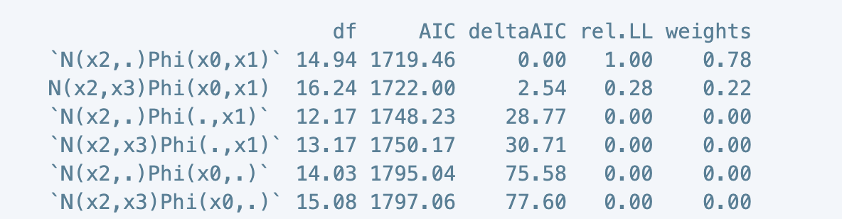
print(models.aictab)
                           df     AIC deltaAIC rel.LL weights
    `N(x2,.)Phi(x0,x1)` 14.94 1719.46     0.00   1.00    0.78
    N(x2,x3)Phi(x0,x1)  16.24 1722.00     2.54   0.28    0.22
    `N(x2,.)Phi(.,x1)`  12.17 1748.23    28.77   0.00    0.00
    `N(x2,x3)Phi(.,x1)` 13.17 1750.17    30.71   0.00    0.00
    `N(x2,.)Phi(x0,.)`  14.03 1795.04    75.58   0.00    0.00
    `N(x2,x3)Phi(x0,.)` 15.08 1797.06    77.60   0.00    0.00
    `N(x2,.)Phi(.,.)`    9.91 1825.14   105.68   0.00    0.00
    `N(x2,x3)Phi(.,.)`  10.95 1827.16   107.70   0.00    0.00
    `N(.,x3)Phi(x0,x1)` 16.15 2938.32  1218.86   0.00    0.00
    `N(.,x3)Phi(.,x1)`  12.42 2965.17  1245.71   0.00    0.00
    `N(.,.)Phi(x0,x1)`   7.03 2989.60  1270.14   0.00    0.00
    `N(.,x3)Phi(x0,.)`  15.24 3013.90  1294.44   0.00    0.00
    `N(.,.)Phi(.,x1)`    3.59 3017.03  1297.57   0.00    0.00
    `N(.,x3)Phi(.,.)`   10.82 3043.42  1323.95   0.00    0.00
    `N(.,.)Phi(x0,.)`    6.13 3065.18  1345.71   0.00    0.00
    `N(.,.)Phi(.,.)`     2.00 3095.28  1375.81   0.00    0.00
The top-performing model is listed here in the first row as N(x2,.)Phi(x0,x1). This model is fully-specified except for the removal of the x3 term in the count portion of the GAM. This model is more parsimonious and is significantly better than the global model, represented in the second row (ΔAIC > 2).
Discussion
In this example, one of the nested models performs significantly better than the global model (ΔAIC > 2), although the global model still has a weight of ~22%. After this, we would be able to use these model weights to calculate model-averaged predictions.
The advantage of model comparison is the ability to make inferences about the effect of individual covariates as well as to make model-averaged predictions. However, if you’re only concerned with inference, the mgcv package includes a useful attribute in the gam() function to address this, which is much more efficient (Huge thanks to Dr. Gavin Simpson for bringing this to my attention via Twitter). By specifying select = TRUE, the gam() function adds selection penalties to the smooth effects, allowing them to be effectively removed from the global model.
testSelect = gam(list(y
                      ~ s(x2) + s(x3),
                      ~ s(x0) + s(x1)),
                 family = ziplss(),
                 gamma = 1.4,
                 select = T)
Once we fit this model, we can interpret the result of select = T by inspecting the effective degrees of freedom (edf). Smooth effects (smoothed covariates) that approach zero are effectively removed from the model through the penalizing process.
summary(testSelect)
Family: ziplss
Link function: identity identity

Formula:
y ~ s(x2) + s(x3)
~s(x0) + s(x1)

Parametric coefficients:
              Estimate Std. Error z value Pr(>|z|)
(Intercept)    1.14782    0.04947  23.205   <2e-16 ***
(Intercept).1 -0.05015    0.06411  -0.782    0.434
---
Signif. codes:  0 ‘***’ 0.001 ‘**’ 0.01 ‘*’ 0.05 ‘.’ 0.1 ‘ ’ 1

Approximate significance of smooth terms:
              edf Ref.df  Chi.sq  p-value
s(x2)   7.1981202      9 1075.34  < 2e-16 ***
s(x3)   0.0002672      9    0.00    0.667
s.1(x0) 3.1043704      9   28.27 5.52e-07 ***
s.1(x1) 0.9809639      9   70.34  < 2e-16 ***
---
Signif. codes:  0 ‘***’ 0.001 ‘**’ 0.01 ‘*’ 0.05 ‘.’ 0.1 ‘ ’ 1

Deviance explained = 61.4%
-REML = 636.54  Scale est. = 1         n = 500
Here we see that s(x3) in the count portion is highly penalized as its edf approaches zero. This agrees with our model comparison table, which found that the model that treated x3 as invariant performed significantly better than the others.
Comparing the AIC scores between the penalized model and this top performing model can provide further support for an agreement between these two methods.
data.frame(AIC(testSelect, `N(x2,.)Phi(x0,x1)`)) %>%
  mutate(model = rownames(.)) %>%
  mutate(deltaAIC = AIC-min(AIC)) %>%
  arrange(AIC) %>%
  select(3,1,2,4)
                model       df      AIC deltaAIC
1 `N(x2,.)Phi(x0,x1)` 14.94116 1719.463 0.000000
2          testSelect 14.71669 1720.730 1.267047
We find that the two models are not significantly different from each other (ΔAIC < 2), meaning that the two methods agree on model structure and result in relatively similar models. Generally, using the penalization method can be a substitute for AIC model comparison if inference is the primary goal. However, conducting the full AIC model comparison process is required to compute model-averaged predictions.
References
-
Akaike, H. Information Theory and an Extension of the Maximum Likelihood Principle. in Proceedings of the Second International Symposium on Information Theory 199–213 (1998).
-
Coelho, M. T. P., Diniz‐Filho, J. A. & Rangel, T. F. A parsimonious view of the parsimony principle in ecology and evolution. Ecography (Cop.). 42, 968–976 (2019).
-
Robinson, O. J. et al. Using citizen science data in integrated population models to inform conservation. Biol. Conserv. 227, 361–368 (2018).
-
Stoica, P. & Söderström, T. On the parsimony principle. Int. J. Control 36, 409–418 (1982).
-
Wood, S. N., Pya, N. & Säfken, B. Smoothing Parameter and Model Selection for General Smooth Models. J. Am. Stat. Assoc. 111, 1548–1563 (2016).