Fast workflow to calculate proportional landcover

Using velox and dplyr to efficiently calculate proportional landcover (‘pland’) in R

Introduction

Environmental covariates are fundamental to spatially-explicit modeling in ecology. There are hundreds of metrics that have been used to characterize and quantify landscapes in ways that are biologically relevant, from average rainfall to net primary production. One such environmental covariate that is particularly popular in distribution modeling is proportional landcover. Calculated using a buffer around each point, this metric describes the composition of the surrounding landscape in terms of the proportion of each represented landcover class. The historical context for this metric comes from the well-known software, FRAGSTATS (McGarigal and Marks 1995), which includes this calculation – termed “pland.”

Now that R is so popular, FRAGSTATS has faded out a bit and has been all but replaced by the R package landscapemetrics. This package offers lots of tools and a straightforward workflow for the analysis of landscapes. The tutorial I’m offering here, though, is a bit more tailored to calculating proportional landcover very efficiently, with a very applicable example using the National Land Cover Database (NLCD). This database is released by USGS and is very commonly used in analysis of landscapes from regions within the United States. One of the strengths of NLCD is that it offers landcover classifications at a very fine spatial resolution of 30m. This resolution surely provides an abundance of information and data to work with, however, it’s computationally intensive. To deal with this, we will implement the R package velox, which was designed to achieve much faster raster extraction operations compared to other solutions within R. Much like the dplyr package, velox can achieve this efficiency by essential serving as a wrapper that conducts the operations in C++.

Methods

Generating sample coordinates

To start, we’ll load the packages the following pacakges for use throughout the walkthrough.

library(dplyr)
library(rnaturalearth)
library(sf)

Jumping into things, we need to get a polygon for Massachusetts, which we can do via the rnaturalearth package. Conveniently, this comes pre-packaged as an sf object, which means we can easily transform its CRS without having to convert the object class. Since we’re dealing with proportional landcover, it’s very important that we use an equal-area projection to maintain comparable buffers around each extraction location. Here we use the Albers Equal Area projection, specified to match the CRS for the nlcd data. For reproducibility, we then sample 10 arbitrary locations from wihtin this polygon to represent the points we intend to use for raster extraction.

state = ne_states(iso_a2 = "US", returnclass = "sf") %>%    # pull admin. bounds. for US
  filter(iso_3166_2 == "US-MA") %>%                         # select Massachusetts
  st_transform(crs = "+proj=aea +lat_1=29.5 +lat_2=45.5 +lat_0=23 +lon_0=-96 +x_0=0 +y_0=0 +ellps=GRS80
+towgs84=0,0,0,0,0,0,0 +units=m +no_defs") # nlcd crs

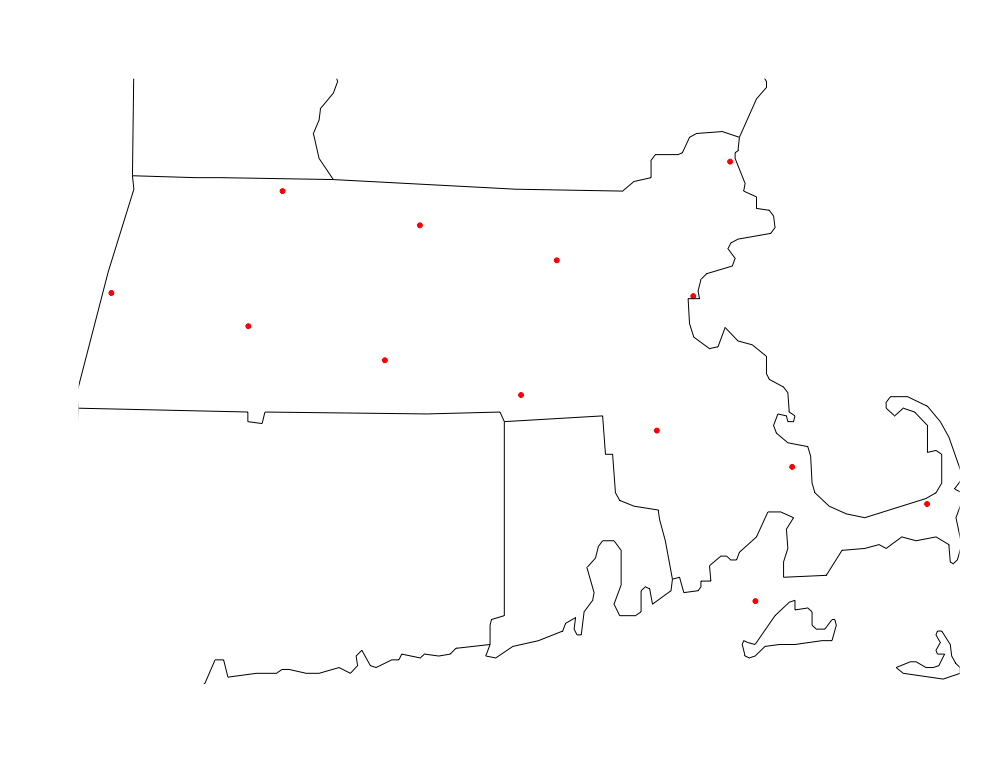
pts = st_sample(state, size = 10, type = "regular")         # sample 10 points in polygon

# Plot!
plot(st_transform(pts, 4326), col="red", pch=20)
maps::map("state", add=T)

Fig. 1: Points plotted in red are locations for raster extraction

Fetching NLCD data

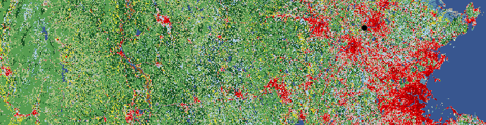
Next we need to get the NLCD data. Luckily, this doesn’t involve any manual downloads or organizing files, etc.; instead, we can use get_nlcd() from the FedData package to do all of the footwork for us.

library(FedData)

nlcd = get_nlcd(        # fn for pulling NLCD data
  template = state,     # polygon template for download
  label = "4pland",     # this is just a character string label
  year = 2011,          # specify the year (2016 should be available soon)
  force.redo = F
) 

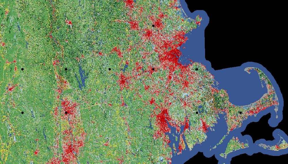
# Plot!
plot(nlcd)
plot(pts, col="black", pch=20, cex=1.5, add=T)

Fig. 2: Points plotted in black are locations for raster extraction

Extract using raster::extract()

Most of us first learn how to do these calculations within the raster package, which we’ll go through here first for comparison to the same process in velox. In raster, this is a very simple operation, where we pass the raster and the points the extract() function, along with a specification for the buffer in meters (1000 m = 1 km). We also specify df = TRUE, so that the output data is a dataframe instead of a list object. This is convenient and straightforward, and works very well for this example, but it is computationally intensive and can be nearly intractable for very large rasters.

library(raster)

ex.mat.r = extract(nlcd, as(pts, 'Spatial'), buffer=1000, df=T) # raster extract

Extract using velox

However, in more complicated analyses with more points and larger areas (read: more pixels), this is where the velox method really shines. First, we convert the raster to a velox object, and then we generate the point-specific buffers and convert them to a spatial polygons data frame, making sure that they all have IDs. At this point, we can now extract pixels within thhe buffers from the raster. This results in a dataframe just like the output from the extract function.

library(velox)
library(sp)

nlcd.vx = velox(stack(nlcd))                                  # raster for velox
sp.buff = gBuffer(as(pts, 'Spatial'), width=1000, byid=TRUE)  # spatial buffer, radius in meters
buff.df = SpatialPolygonsDataFrame(
            sp.buff,                                         
            data.frame(id=1:length(sp.buff)),                 # set ids
            FALSE)                                            # df of buffers
ex.mat.vx = nlcd.vx$extract(buff.df, df=T)                    # extract buffers from velox raster
rm(nlcd.vx) # removing the velox raster can free up space

Calculate pland

No matter which method you choose, dplyr is a great choice for carrying out the pland calculations, which you can see below. Compared to what would otherwise be a mess of nested for and if loops, this workflow is far more streamlined and easier to follow, and takes much less time.

prop.lc = ex.mat.vx %>%
  setNames(c("ID", "lc_type")) %>%        # rename for ease
  group_by(ID, lc_type) %>%               # group by point (ID) and lc class 
  summarise(n = n()) %>%                  # count the number of occurences of each class
  mutate(pland = n / sum(n)) %>%          # calculate percentage
  ungroup() %>%                           # convert back to original form
  dplyr::select(ID, lc_type, pland) %>%   # keep only these vars
  complete(ID, nesting(lc_type), 
  fill = list(pland = 0)) %>%             # fill in implicit landcover 0s
  spread(lc_type, pland)                  # convert to long format

Assign landcover class names

Finally, for convenience, we can map the landscape class numbers back to their original names. This part is a bit in-the-weeds, but it makes any following analyses far easier. In the code below, we pull a hash table form the nlcd object and then use merge.data.frame() to match values from the hash table to the dataframe containing the pland values. merge.data.frame() is an extremely useful function, similar to VLOOKUP in Excel, amd has been designed for exactly this purpose of mapping values from one dataframe to another,

nlcd_cover_df = as.data.frame(nlcd@data@attributes[[1]]) %>%      # reference the name attributes
  subset(NLCD.2011.Land.Cover.Class != "") %>%                    # only those that are named
  dplyr::select(ID, NLCD.2011.Land.Cover.Class)                   # keep only the ID and the lc class name
lc.col.nms = data.frame(ID = as.numeric(colnames(prop.lc[-1])))   # select landcover classes
matcher = merge.data.frame(x = lc.col.nms,                        # analogous to VLOOKUP in Excel
                           y = nlcd_cover_df,
                           by.x = "ID",
                           all.x = T)               
colnames(prop.lc) = c("ID", as.character(matcher[,2]))            # assign new names

Results

This looks great. For a quick checking, summing the values for each row across the columns should add up to 1, which looks right from a quick check!

print(prop.lc)

# A tibble: 9 x 16
  ID    `Open Water` `Developed, Ope… `Developed, Low… `Developed, Med… `Developed, Hig… `Barren Land`
  <fct>        <dbl>            <dbl>            <dbl>            <dbl>            <dbl>         <dbl>
1 1          0                 0.288           0.314            0.300           0.0437         0.00175
2 2          0.00729           0.132           0.103            0.0545          0.00933        0      
3 3          0.0140            0.130           0.0998           0.0692          0.0131         0.00146
4 4          0.00320           0.0300          0.0116           0.00146         0              0      
5 5          0.00291           0.0921          0.0752           0.0807          0.0245         0      
6 6          0.257             0.0364          0.105            0.0489          0.000582       0.143  
7 7          0.00320           0.0501          0.00815          0.00844         0              0      
8 8          0.00292           0.128           0.151            0.0814          0.00787        0      
9 9          0.991             0               0                0               0              0.00437
# … with 9 more variables: `Deciduous Forest` <dbl>, `Evergreen Forest` <dbl>, `Mixed Forest` <dbl>,
#   `Shrub/Scrub` <dbl>, Herbaceuous <dbl>, `Hay/Pasture` <dbl>, `Cultivated Crops` <dbl>, `Woody
#   Wetlands` <dbl>, `Emergent Herbaceuous Wetlands` <dbl>

I hope this has been tutorial has provided a convenient and straightforward demonstration of how velox can fit into your workflow!

References

McGarigal, K. andBJ Marks. 1994. FRAGSTATS v2: Spatial Pattern Analysis Program for Categorical and Continuous Maps. Computer software program produced by the authors at the University of Massachusetts, Amherst. Available at the following web site: http://www.umass.edu/landeco/research/fragstats/fragstats.html